Mathematics of Deep Learning Notes

By Bolun Dai | Feb 27th 2021

The blog is derived from the notes I have from taking the Mathematics of Deep Learning course by Joan Bruna at New York Univeristy.

Main Ingredients of Superivised Learning

A supervised learning problem usually consists of four components: the input domain \(\chi\), the data distribution \(\nu\), the target function \(f^*\) and a loss (or risk) \(\mathcal{L}\).

The input domain \(\chi\) is usually high dimension, \(\chi\in\mathbb{R}^d\). For the MNIST dataset, inputs are of dimension \(28\times28 = 784\). The data distribution \(\nu\) is defined over an input domain \(\chi\), \(\nu\in P(\chi)\), where \(P(\chi)\) is the set of all probability distributions over the input domain \(\chi\). The target function \(f^*\) maps inputs to scalar values, \(f^*: \chi\rightarrow\mathbb{R}\), i.e. for an image \(\chi_i\), \(f^*\) maps it to \(1\) if it contains a cat, \(0\) otherwise. The loss (or risk) \(\mathcal{L}\) is a functional

\[\mathcal{L}(f) = \mathbb{E}_{x\sim\nu}\Big[\ell\Big(f(x), f^*(x)\Big)\Big],\]

this is saying for data sampled from data distribution \(\nu\) the loss is a metric of the difference between the learned function \(f\) and target function \(f^*\). For mean squared error (MSE) loss, we have

\[\mathcal{L}(f) = \mathbb{E}_{x\sim\nu}\Big[\Big|f(x) - f^*(x)\Big|^2\Big] = \Big\|f(x) - f^*(x)\Big\|_\nu^2,\]

here the loss \(\mathcal{L}\) is convex w.r.t the learned function \(f\).

The goal of supervised learning is to predict the target function \(f^*\) from finite number of observations, under the assumption observations are sampled i.i.d from the data distribution \(\nu\)

\[\nu = \Big\{\Big(x_i, f^*(x_i)\Big)\Big\}_i,\ x_i\underset{iid}{\sim}\nu.\]

Since we cannot know exactly how well an algorithm will work in practice (the true “risk”) because we don’t know the true distribution of data that the algorithm will work on, we can instead measure its performance on a known set of training data (the “empirical” risk) (Wikipedia). The empirical risk is defined as

\[\widehat{\mathcal{L}}(f) = \frac{1}{L}\sum_{i=1}^{L}\ell\Big(f(x), f^*(x)\Big).\]

Instead of looking at any function \(f\) we are only searching for the target functions within a subset. We consider a hypothesis space of possible functions that approximates the target function

\[\mathcal{F} \subseteq \Big\{f: \chi\rightarrow\mathbb{R}\Big\},\]

where it is a normed space. By saying it is a norm space we are saying a measurement of length exists, in this case the “length” measurement denotes the complexity of the function. Thus, \(\gamma: \mathcal{F}\rightarrow\mathbb{R}\), where \(\gamma(f)\) denotes how complex the hypothesis \(f\in\mathcal{F}\) is. In the case of deep learning, \(\mathcal{F}\) can be the set of neural networks of a certain architecture, i.e.

\[\mathcal{F} = \Big\{f: x\rightarrow\mathbb{R}\ \Big|\ f(x) = w_3g_2(w_2g_1(w_1x))\Big\},\]

where \(w_i\) is the weight vector of the \(i\)-th layer and \(g_i\) is the \(i\)-th activation function. This denotes the set of neural networks with three layers, no bias and two activation functions (no activation at the output layer). If we consider a ball

\[\mathcal{F}_\delta = \Big\{f\in\mathcal{F}\ \Big|\ \gamma(f)\leq\delta\Big\},\]

it is a convex set, we can then only look for functions within this ball.

Now the principle of stuctural risk minimization can be introduced. When fitting a function to a dataset overfitting can occur, this usually happens when the learned function has high complexity. When overfitting occurs, the learned model will have a really good performance on the training set and will generally perform badly on the test set. Therefore, to avoid overfitting, we would like the learned model to have low complexity while minimizing the training error. These two objectives can be written as

\[\min_{\gamma(f)\leq\delta}\widehat{\mathcal{L}}(f),\]

this is called the constrained form, where the emprical risk is minimized while restricting the complexity of the learned model. We can also write it in the penalized form

\[\min_{f\in\mathcal{F}}\widehat{\mathcal{L}}(f) + \lambda\gamma(f),\]

to penalize models with large complexity. Or the interpolating form

\[\begin{align*} \min &\ \gamma(f)\\ \mathrm{s.t.} &\ \widehat{\mathcal{L}}(f) = 0. \end{align*}\]

Note the interpolating form makes sense only when the data has no false labels.

Basic Decomposition of Errors

Suppose using the constrained form we found a function \(\tilde{f}\in\mathcal{F}_\delta\), such that

\[\widehat{\mathcal{L}}(\tilde{f}) \leq \min_{f\in\mathcal{F}_\delta}\widehat{\mathcal{L}}(f) + \epsilon_o.\]

This is saying the empirical loss of the candidate function \(\tilde{f}\) is only \(\epsilon_0\) away from the best solution in the ball (the problem is almost solved). Now let’s take a look at how good is our candidate function \(\tilde{f}\) w.r.t. to the original loss (not the empirical loss)

\[\begin{align*} &\ \mathcal{L}(\tilde{f}) - \min_{f\in\mathcal{F}}\mathcal{L}(f)\\ =&\ \mathcal{L}(\tilde{f}) - \min_{f\in\mathcal{F}_\delta}\mathcal{L}(f) + \min_{f\in\mathcal{F}_\delta}\mathcal{L}(f) - \min_{f\in\mathcal{F}}\mathcal{L}(f)\\ =&\ \mathcal{L}(\tilde{f}) - \min_{f\in\mathcal{F}_\delta}\mathcal{L}(f) + \epsilon_a & \epsilon_a = \min_{f\in\mathcal{F}_\delta}\mathcal{L}(f) - \min_{f\in\mathcal{F}}\mathcal{L}(f)\\ =&\ \widehat{\mathcal{L}}(\tilde{f}) - \min_{f\in\mathcal{F}_\delta}\mathcal{L}(f) + \mathcal{L}(\tilde{f}) - \widehat{\mathcal{L}}(\tilde{f}) + \epsilon_a\\ \leq&\ \min_{f\in\mathcal{F}_\delta}\widehat{\mathcal{L}}(f) - \min_{f\in\mathcal{F}_\delta}\mathcal{L}(f) + \mathcal{L}(\tilde{f}) - \widehat{\mathcal{L}}(\tilde{f}) + \epsilon_a + \epsilon_o & \text{used inequality above}\\ \leq&\ 2\sup_{f\in\mathcal{F}_\delta}\Big|\mathcal{L}(f) - \widehat{\mathcal{L}}(f)\Big| + \epsilon_a + \epsilon_o & \text{see proof below}\\ =&\ \epsilon_s + \epsilon_a + \epsilon_o & \epsilon_s = 2\sup_{f\in\mathcal{F}_\delta}\Big|\mathcal{L}(f) - \widehat{\mathcal{L}}(f)\Big| \end{align*}\]

We now see why

\[\min_{f\in\mathcal{F}_\delta}\widehat{\mathcal{L}}(f) - \min_{f\in\mathcal{F}_\delta}\mathcal{L}(f) \leq \sup_{f\in\mathcal{F}_\delta}\Big|\mathcal{L}(f) - \widehat{\mathcal{L}}(f)\Big|.\]

Assume we have

\[\DeclareMathOperator*{\argmin}{arg\,min} \argmin_{f\in\mathcal{F}_\delta}\widehat{\mathcal{L}}(f) = f_1\ \ \ \text{and}\ \ \ \argmin_{f\in\mathcal{F}_\delta}\mathcal{L}(f) = f_2.\]

For the case

\[\min_{f\in\mathcal{F}_\delta}\widehat{\mathcal{L}}(f) > \min_{f\in\mathcal{F}_\delta}\mathcal{L}(f),\]

we have

\[\begin{align*} \min_{f\in\mathcal{F}_\delta}\widehat{\mathcal{L}}(f) - \min_{f\in\mathcal{F}_\delta}\mathcal{L}(f) &= \widehat{\mathcal{L}}(f_1) - \mathcal{L}(f_2)\\ &\leq \widehat{\mathcal{L}}(f_2) - \mathcal{L}(f_2)\\ &\leq \sup_{f\in\mathcal{F}_\delta}\Big|\mathcal{L}(f) - \widehat{\mathcal{L}}(f)\Big|, \end{align*}\]

which is denoted by the right figure.

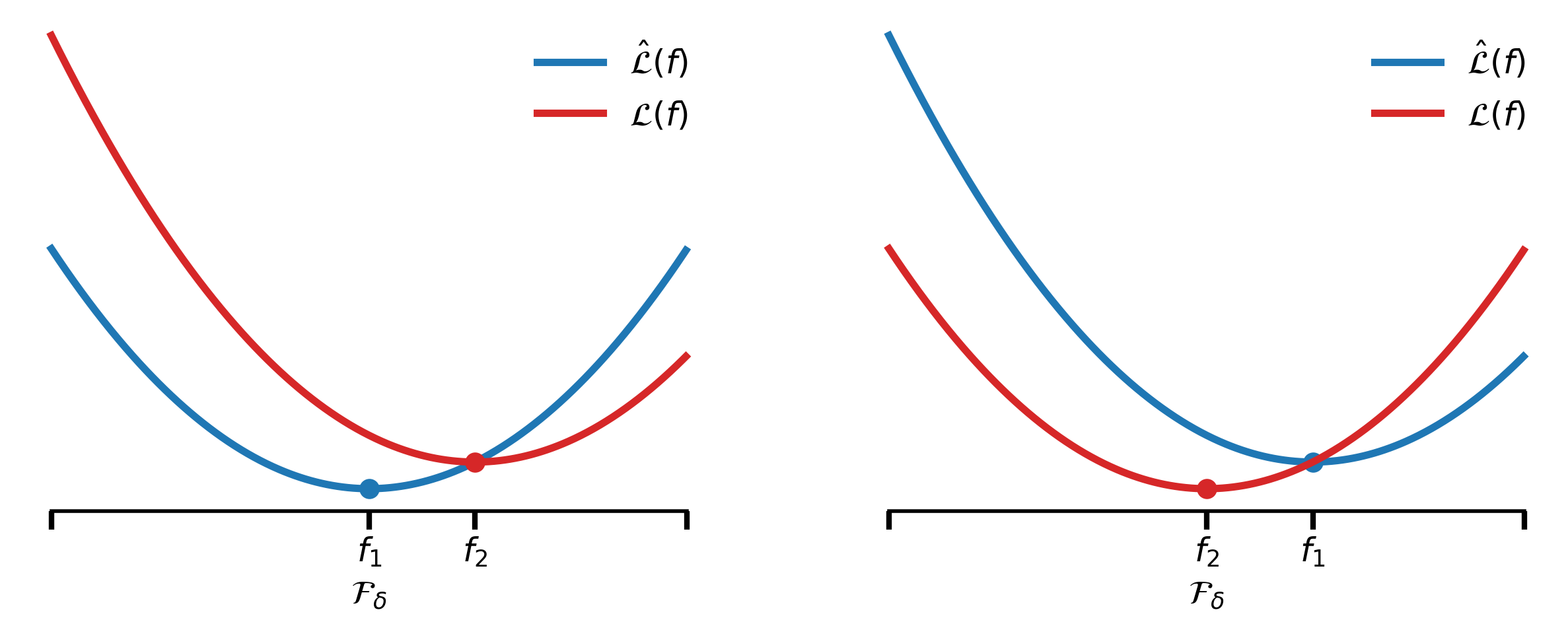
For the case

\[\min_{f\in\mathcal{F}_\delta}\widehat{\mathcal{L}}(f) \leq \min_{f\in\mathcal{F}_\delta}\mathcal{L}(f),\]

we have

\[\min_{f\in\mathcal{F}_\delta}\widehat{\mathcal{L}}(f) - \min_{f\in\mathcal{F}_\delta}\mathcal{L}(f) \leq 0 \leq \sup_{f\in\mathcal{F}_\delta}\Big|\mathcal{L}(f) - \widehat{\mathcal{L}}(f)\Big|,\]

which is denoted by the left figure. Thus we have

\[\min_{f\in\mathcal{F}_\delta}\widehat{\mathcal{L}}(f) - \min_{f\in\mathcal{F}_\delta}\mathcal{L}(f) \leq \sup_{f\in\mathcal{F}_\delta}\Big|\mathcal{L}(f) - \widehat{\mathcal{L}}(f)\Big|.\]

Now let’s take a look at each of the three errors: approximation error \(\epsilon_a\), statisical error \(\epsilon_s\) and optimization error \(\epsilon_o\). We have the approximation error as

\[\begin{align*} \epsilon_a &= \min_{f\in\mathcal{F}_\delta}\mathcal{L}(f) - \min_{f\in\mathcal{F}}\mathcal{L}(f)\\ &= \min_{f\in\mathcal{F}_\delta}\|f - f^*\|_2^2 - \min_{f\in\mathcal{F}}\|f - f^*\|_2^2. \end{align*}\]

The first term is the approximation error of the set of functions \(f\in\mathcal{F}_\delta\). The second term is the approximation error using any function \(f\). Using the universal approximation theorem we know for neural networks of more than two layers the second term is equal to \(0\). Thus we have

\[\epsilon_a = \min_{f\in\mathcal{F}_\delta}\mathcal{L}(f),\]

which decreases as \(\delta\) increases. The optimization error \(\epsilon_o\) is present due to the use of algorithms such as SGD and ADAM when finding the weights of a neural network. The statisical error \(\epsilon_s\) has the form of

\[\epsilon_s = 2\sup_{f\in\mathcal{F}_\delta}\Big|\mathcal{L}(f) - \widehat{\mathcal{L}}(f)\Big| \sim O\Big(\sqrt{\frac{\delta}{L}}\Big),\]

where \(\delta\) represents the complexity and \(L\) represents the number of samples. To understand this we can write out the two terms \(\mathcal{L}(f)\) and \(\widehat{\mathcal{L}}(f)\) as

\[\mathcal{L}(f) = \mathbb{E}_{x\sim\nu}\Big[f(x)\Big]\ \ \ \text{and}\ \ \ \widehat{\mathcal{L}}(f) = \widehat{\mathbb{E}}_{x\sim\nu}\Big[f(x)\Big].\]

From the law of big numbers we know that when the number of samples \(L\) is large we have \(\mathcal{L}(f) \approx \widehat{\mathcal{L}}(f)\), thus small statisitical error \(\epsilon_s\). Note \(\epsilon_s\) is not about a single function \(f\in\mathcal{F}_\delta\) but all of the function in \(\mathcal{F}_\delta\). Therefore, if \(\delta\) increases the number of functions that belongs to the set \(\mathcal{F}_\delta\) also increases. Thus making the statisical error \(\epsilon_s\) larger.

Curse of Dimensionality

This section will discuss how approximation error \(\epsilon_a\), statisical error \(\epsilon_s\) and optimization error \(\epsilon_o\) will behave as the input dimension changes.

First, let’s talk about the statisitical curse. Assume we observe \(\{x_i, f^*(x_i)\}_i\), for \(i = 1, \cdots, L\) and \(x_R\in\mathbb{R}^d\). The question we would like to ask is for \(f^*\) belonging to a certain hypothesis class and the dimension of the input \(d\), what is the number of observations \(L\) required to estimate \(f^*\) up to a certain accuracy.

Suppose the target function \(f^*\) is a linear function: \(f^*(x) = x^T\theta\), \(\theta\in\mathbb{R}^d\), then instead of looking into all classes of functions, the hypothesis space would only include linear functions

\[\mathcal{F} = \Big\{f: \mathbb{R}^d\rightarrow\mathbb{R}\ \Big|\ f(x) = x^T\theta\Big\}.\]

Now the function is parametrized by a \(d\)-dimension vector, since it is a linear function we can treat the observations as \(L\) linear equations with \(d\) unknowns

\[\Big\{x_i^T\theta_\mathrm{est} = f^*(x_i)\Big\}_{i = 1 \sim L}.\]

From our knowledge of linear algebra we know that as long as \(L\geq d\) we can find a definitive solution.

What about functions that are only locally linear? A function that is locally linear can be defined as

\[\|f(x) - f(\tilde{x})\| \leq \beta\|x - \tilde{x}\|,\]

which is the same as being \(\beta\)-Lipschitz. Thus, the function space we search for is

\[\mathcal{F} = \Big\{f: \mathbb{R}^d\rightarrow\mathbb{R}\ \Big|\ f\ \text{is Lipschitz}\Big\}.\]

For this class a functions a good candidate for determining the complexity is something like the variance in curvature. We don’t want the function to be very curly. To describe this mathematically we can use the Lipschitz constant

\[\gamma(f) = \mathrm{Lip}(f) + \|f\|_\infty,\]

I am not sure why the second term is there, but that does not interfere with the intuition provided. Just to restate the goal \(\forall\epsilon\), we would like to find \(f\in\mathcal{F}\), such that \(\|f - f^*\|\leq\epsilon\), from \(L\) i.i.d samples \(\{x_i, f^*(x_i)\}_{i=1\sim L}\). And the question would be how large of a \(L\) would be required to achieve error \(\epsilon\). The answer is \(L\sim\epsilon^{-d}\). To find such a function we would basically need to grid the domain, therefore for a \(1\)-dimension hypercube we would need \(1/\epsilon = \epsilon^{-1}\) samples to achieve accuracy \(\epsilon\), for a \(2\)-dimension problem we would need \(\epsilon^{-2}\) samples and for a \(d\)-dimension problem it would require \(\epsilon^{-d}\) samples. Now let’s prove that this is in fact the upper bound of the number of samples required to achieve error \(\epsilon\). Given \(\{x_i, f^*(x_i)\}_{i=1\sim L}\), consider

\[\DeclareMathOperator*{\argmin}{arg\,min} \hat{f} = \argmin_{f\in\mathcal{F}}\Big\{\mathrm{Lip}(f)\ \Big|\ f(x_i) = f^*(x_i), \forall i\Big\},\]

and assume \(\mathrm{Lip}(f^*) = 1\). Then we can say \(\mathrm{Lip}(\hat{f}) \leq 1\), because we already know that a function with Lipschitz coefficient \(1\) goes through all of the points and \(\hat{f}\) is the function with the smallest Lipschitz coefficient that goes through all of the points. Thus, we have \(\mathrm{Lip}(\hat{f}) \leq \mathrm{Lip}(f^*) = 1\). For a random data point \(x\) and \(\bar{x}\) being the training data closest to \(x\) we have

\[\begin{align*} |\hat{f}(x) - f^*(x)| &= |\hat{f}(x) - f^*(x) - \hat{f}(\bar{x}) + \hat{f}(\bar{x}) - f^*(\bar{x}) + f^*(\bar{x})|\\ &\leq |\hat{f}(x) - \hat{f}(\bar{x})| + |\hat{f}(\bar{x}) - f^*(\bar{x})| + |f^*(\bar{x}) - f^*(x)|\\ &= |\hat{f}(x) - \hat{f}(\bar{x})| + |f^*(\bar{x}) - f^*(x)| & \hat{f}(\bar{x}) - f^*(\bar{x}) = 0\\ &\leq 2\|x - \bar{x}\| & \mathrm{Lip}(\hat{f}) \leq \mathrm{Lip}(f^*) = 1 \end{align*}\]

If we take the expectation of the square on both sides we have

\[\mathbb{E}_{x\sim\nu}\Big[|\hat{f}(x) - f^*(x)|^2\Big] \leq \mathbb{E}_{x\sim\nu}\Big[4\|x - \bar{x}\|^2\Big] = w_2^2(\nu, \hat{\nu}_L) \sim L^{-1/d} = \epsilon,\]

this is saying the square expectation has the same representation as the wassertein distance between the real data distribution \(\nu\) and the empirical data distribution for \(L\) samples \(\hat{\nu}_L\). Such a wassertein distance is on the order of \(L^{-1/d}\). Then we have

\[L^{-1/d} = \epsilon\ \rightarrow\ L = \epsilon^{-d}.\]

Also using maximum descrepancy (did not go into detail) one can establish the lower bound is also \(\epsilon^{-d}\), this means unless we grid the domain little can be done.

To summarize, for linear functions we would only need a small amount of samples but this set of functions can be too restricitive, while looking a Lipschitz functions we would need exponentionally more samples, which is simply too much. Therefore, the majority of the functions discussed in this set of notes will be between these two categories.

Now let’s talk about the curse of dimensionality in approximation. To state the results, for smooth functions we can get a nice approximation with small neural networks. Where for functions that are not very smooth we would need an infinite number of neurons.

For the curse of dimensionality in optimization we would also need to grid the domain, which requires an exponentional number of operations. One set of functions that breaks this curse is convex functions.