Cart-pole Swing-up Task Using MPC
By Bolun Dai | Apr 20th 2022
In this blog, I want to swing up a cart-pole system using a model predictive control (MPC) based method. When I was initially shown this problem, I thought it was a toy problem and that I would be able to solve it in a few minutes. Then I realized that in school, all I had been taught was linear MPC, and for cartpole-related problems, all I knew was how to balance it at the top, assuming that it started close to the top so that the linearization is still valid. As for the case of swinging up the cartpole, this sits firmly in the realm of nonlinear control, which I have also learned about. One of the more classical ways to deal with this would then be to linearize along the trajectory, such as using iLQR. However, when given state and control constraints, e.g., limits on control effort and not letting the cartpole sway too far, iLQR loses its appeal. There are ways to incorporate constraints into iLQR, such as
I then did some reading and I found a way to do constrained nonlinear control: using direct collocation
Introduction
Now let’s first define the system and the problem. The dynamics of the cart-pole system can be defined as
\[\dot{\mathbf{x}} = \begin{bmatrix} \dot{x}\\ \dot{\theta}\\ \ddot{x}\\ \ddot{\theta} \end{bmatrix} = \begin{bmatrix} \dot{x}\\ \dot{\theta}\\ \frac{m_p\sin{\theta}(l\dot{\theta}^2 + g\cos{\theta})}{m_c + m_p\sin^2{\theta}}\\ \frac{-m_pl\dot{\theta}^2\cos{\theta}\sin{\theta} - (m_c + m_p)g\sin{\theta}}{l(m_c + m_p\sin^2{\theta})} \end{bmatrix} + \begin{bmatrix} 0\\ 0\\ \frac{1}{m_c + m_p\sin^2{\theta}}\\ \frac{-1}{l(m_c + m_p\sin^2{\theta})} \end{bmatrix}u,\]where \(m_c\) is the weight of the cart, \(m_p\) is the weight of the pole, \(\ell\) is the length of the pole, \(x\) is the center-of-mass position of the cart, \(\theta\) is the orientation of the pole, and \(u\) is the control action, which in this case is a force acting on the cart. The control problem is to swing up the pole until it balances at the upright position. This can be captured using the following cost function
\[J = \int_{0}^{T}{(\mathbf{x}(t) - x^*)^TQ(\mathbf{x}(t) - x^*) + u(t)^TRu(t)dt},\]where \(Q\) and \(R\) are weight matrices, \(T\) is the preview horizon, and \(x^*\) is the target state, which in this case is \([1,\ \pi,\ 0,\ 0]^T\). To make the problem more realistic, the cart position and control efforts are all constrained, i.e., \(x\in[-a,\ a]\) and \(u\in[-b,\ b]\). This problem is a nonlinear constrained optimization problem, which is quite hard to solve; if written as-is, I don’t even know how to give it to a solver (if anyone reading this has a solution, please let me know). In the next section, we will look into how, using a trapezoidal collocation method, we can transform the problem into something more tractable.
Trapezoidal Collocation
The key idea here is to approximate integrals using trapezoidal quadrature. There are other ways to approximate it, as mentioned in
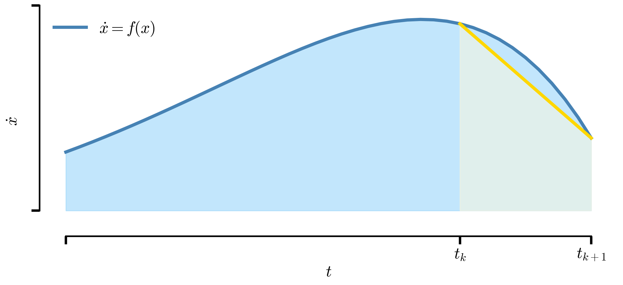
Here we can use the system dynamics \(\dot{x} = f(x)\) as an example. If we want to integrate the system dynamics from \(t_k\) to \(t_{k+1}\),
\[\int_{t_k}^{t_{k+1}}{\dot{x}} = \int_{t_k}^{t_{k+1}}{f(x)},\]this is equivalent to calculating the area under the curve \(f(x)\) from \(t_k\) to \(t_{k+1}\), which we can easily see can be approximated by a trapezoidal quadrature denoted by the yellow region. Using the formula for trapezoidal area, we can get an approximation of the system dynamics
\[\int_{t_k}^{t_{k+1}}{\dot{x}} = \frac{t_{k+1} - t_k}{2}\Big(f(x(t_k)) + f(x(t_{k+1}))\Big) \approx x(t_{k+1}) - x(t_k),\]where the last approximation is obtained by the fundamental theorem of calculus. By discretizing the system dynamics and cost function using a trapezoidal approximation, we can easily write out the aforementioned nonlinear constrained optimization problem, which we will discuss in the next section.
Reformulation
Using the aforementioned trapezoidal approximation, we can transform the cost from an integration over the entire trajectory into a summation at a few states, which are called knot points. The step-wise cost is
\[w(t) = (\mathbf{x}(t) - x^*)^TQ(\mathbf{x}(t) - x^*) + u(t)^TRu(t).\]If we take the integral between \(t_k\) and \(t_{k+1}\), we have
\[\int_{t_k}^{t_{k+1}}{w(t)dt} \approx \frac{t_{k+1} - t_k}{2}\Big(w(t_k) + w(t_{k+1})\Big).\]If we pick a series of timesteps \(h_k = t_{k+1} - t_k\), then for the entire preview horizon we can have
\[\int_{0}^{T}{w(t)dt} = \sum_{i=0}^{N-1}{\frac{h_k}{2}\Big(w(t_k) + w(t_{k+1})\Big)}.\]Similarly, to ensure that the state dynamics are respected, an equality constraint needs to be added. Following the same formulation as in the last section, we have a set of equality constraints, one at each knot point,
\[\frac{h_k}{2}\Big(f(x(t_k)) + f(x(t_{k+1}))\Big) = x(t_{k+1}) - x(t_k), \forall i = 1, \cdots, N-1.\]Now we can write out the reformulated problem:
\[\begin{align*} \min_{x(\cdot), u(\cdot)}\ &\ \sum_{i=0}^{N-1}{\frac{h_k}{2}\Big(w(t_k) + w(t_{k+1})\Big)}\\ s.t.\ &\ \frac{h_k}{2}\Big(f(x(t_k)) + f(x(t_{k+1}))\Big) = x(t_{k+1}) - x(t_k)\\ &\ -\mathbf{a} \leq x(t_k) \leq \mathbf{a}\\ &\ -b \leq u(t_k) \leq b.\\ &\ x_0 = 0, \forall i = 1, \cdots, N-1. \end{align*}\]For the original direct collocation approach, the cost is only the control squared, and there is an additional terminal state constraint. However, in an MPC framework, this approach is too “fragmented”. Intuitively, one can think that under such a setup, in order to minimize the cost, it would be best to plan to only reach the top at the end of the preview horizon. Since in MPC the preview horizon is moving, this will make the system never actually attempt to reach the target, but always “prepare” to.
Results
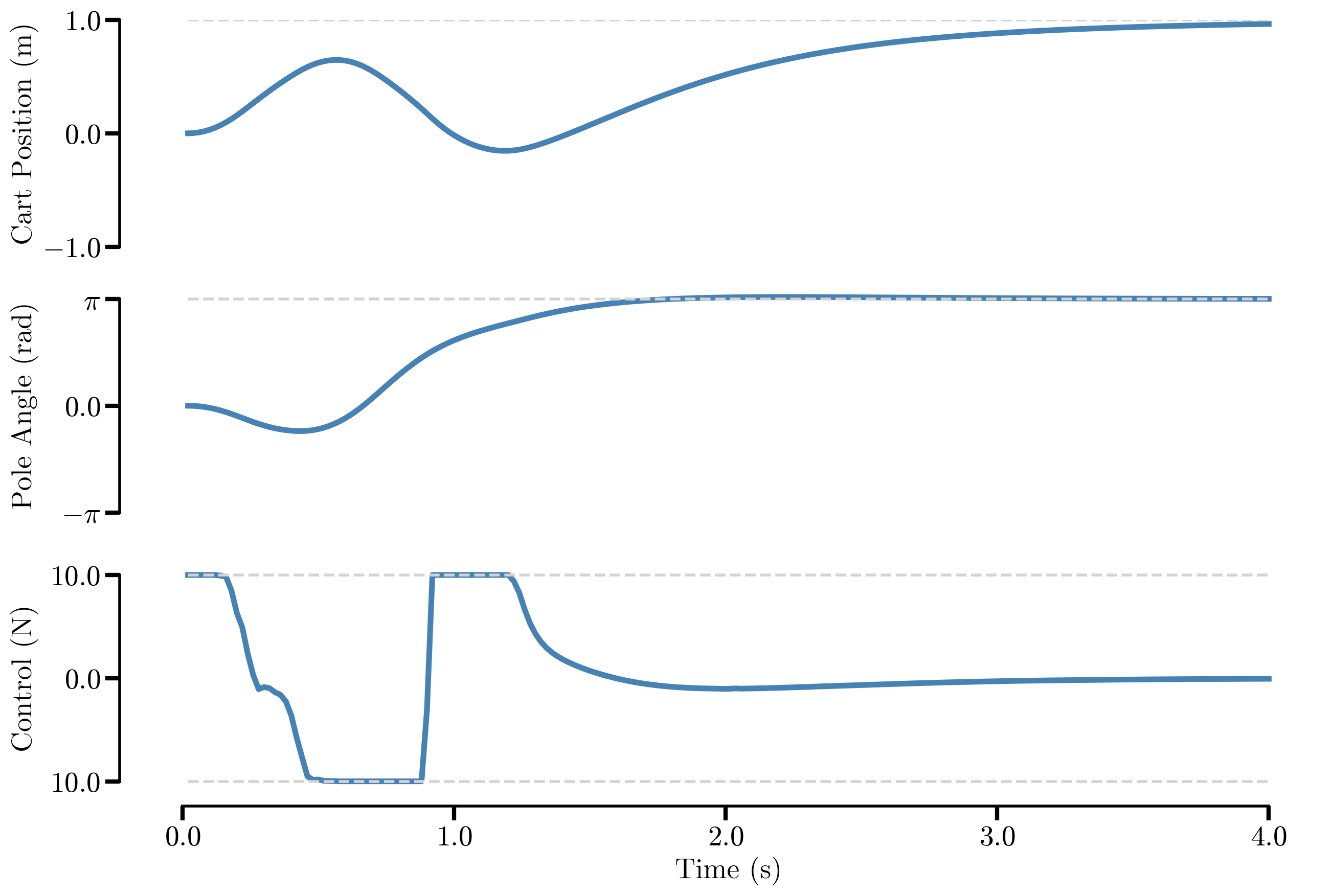
Using the aforementioned approach, we can see that the cart-pole system is able to balance at the top. The control is saturated at 10N. The target is \([1.0,\ \pi,\ 0.0,\ 0.0]\). Though not shown here, the simulation was run for 10 seconds and the pole is firmly balanced at the top. We see that this approach truly is able to solve the cartpole swing-up task. One thing to note is that when running SQP, there is no need to run until a solution is found; in this case, only four iterations are allowed at each timestep.
A few notes on the implementation. I implemented this in Matlab, since I was unable to get scipy’s optimization package to work, while fmincon works right out of the box — credit to Mathworks. If anyone is able to get this working with scipy, please let me know; I am dying to know what I did wrong. To ensure the system dynamics are as close to reality as possible, they were integrated using ode45. This shows that even though the dynamics are simplified when using trapezoidal collocation, the resulting control is still adequate in dealing with real dynamics.
Powered by
![]()