Introduction to Rigid Transformations

By Bolun Dai | Apr 20th 2022

In this blog, I want to give a review of rigid transformations, specifically rotation and translation. Although this is one of the most basic concepts in robotics, I tend to confuse many of these concepts. Therefore, this to me is more like a cheat sheet. The content is developed from .

Rigid Transformations

A rigid transformation in \(\mathbb{R}^3\) is a mapping \(g:\mathbb{R}^3\rightarrow\mathbb{R}^3\) that has the following properties:

Length is preserved: \(\|g(p) - g(q)\| = \|p - q\|\) for all points \(p, q\in\mathbb{R}^3\).
The cross product is preserved: \(g_*(v\times w) = g_*(v)\times g_*(w)\) for all vectors \(v, w\in\mathbb{R}^3\).

In addition to the above properties, we can also prove that the inner product is preserved: \(v_1^Tv_2 = g_*(v_1)^Tg_*(v_2).\)

We can see from the above animation that, after translation and rotation, the length of the two blue lines did not change (\(\|\cdot\|\) did not change), thus satisfying the first property. From the definition of the inner product, we have

\[\langle \mathbf{a}, \mathbf{b}\rangle = \|\mathbf{a}\|\|\mathbf{b}\|\cos(\theta),\]

where \(\theta\) is the angle between \(\mathbf{a}\) and \(\mathbf{b}\). We can see that the angle between the two lines did not change (\(\cos(\theta)\) does not change), and since the length is also kept the same, the inner product is preserved. The rotation is in a 2D plane, but we can see that for the body coordinate system before and after the transformation (orange axes), the z-axis is the same, thus the cross product is preserved. This result generalizes to 3D rotations.

Rotations

Properties

The rotation matrix has the following properties: \(SO(3) = \{R\in\mathbb{R}^{3\times3}\ |\ RR^T = I, \mathrm{det}R = 1\},\)

where \(SO(3)\) represents the special orthogonal group. Since the rotation matrices form a group under matrix multiplication, they have some additional properties:

Closure: if \(R_1, R_2\) are rotation matrices, then \(R_1R_2\) is also a rotation matrix.
Identity: the identity matrix is the identity element.
Inverse: each rotation matrix has an inverse \(R^{-1} = R^T\).
Associativity: for rotation matrices \(R_1, R_2\), and \(R_3\), we have \((R_1R_2)R_3 = R_1(R_2R_3)\).

Also, a rotation matrix is a rigid transformation, which means that

\(R\) preserves length: \(\|Rq - Rp\| = \|p - q\|\) for all points \(p, q\in\mathbb{R}^3\).
\(R\) preserves orientation: \(R(v\times w) = (Rv)\times(Rw)\) for all vectors \(v, w\in\mathbb{R}^3\).

Representations

We can see from the animation that if we have a vector \(\mathbf{q}\) rotating with respect to another vector \(\omega\) with constant angular velocity \(\|\omega\|\), its linear velocity can be calculated as \(\dot{\mathbf{q}} = \omega\times\mathbf{q} = \hat{\omega}\mathbf{q}\). From our knowledge of linear systems (the solution of \(\dot{x} = Ax\) is \(x(t) = e^{At}x_0\)), we have the trajectory of the vector as \(\mathbf{q}^\prime = \mathbf{q}(t) = e^{\hat{\omega}t}\mathbf{q}_0\). Additionally, if we have \(\|\omega\| = 1\), then \(t = \theta\), the rotation angle.

From Euler’s theorem, we know that for any rotation matrix \(R\in SO(3)\), it can be seen to be equivalent to rotation about a fixed axis \(\omega\in\mathbb{R}^3\) through an angle \(\theta\in[0, 2\pi]\). To represent the rotation matrix this way, we can use the exponential map

\[R = e^{\hat{w}\theta} = I + \frac{\hat{\omega}}{\|\omega\|}\sin{(\|\omega\|\theta)} + \frac{\hat{\omega}^2}{\|\omega\|}\bigg(1 - \cos{((\|\omega\|\theta))}\bigg)\]

where \(\hat{\omega}\) is defined as

\[\hat{\omega} = \begin{bmatrix} 0 & -\omega_3 & \omega_2\\ \omega_3 & 0 & -\omega_1\\ -\omega_2 & \omega_1 & 0 \end{bmatrix}\in so(3) = \{S\in\mathbb{R}^{3\times3}\ |\ S^T = -S\}.\]

This mapping is many-to-one, which says that there are many \(e^{\hat{w}\theta}\) corresponding to one \(R\); for every \(R\in SO(3)\), we have more than one \(e^{\hat{w}\theta}\). To obtain \(\omega\) and \(\theta\) from \(R\), we have

\[\theta = \cos^{-1}\Big(\frac{\mathrm{trace}(R) - 1}{2}\Big)\ \mathrm{and}\ \omega = \frac{1}{2\sin\theta}\begin{bmatrix} r_{32} - r_{23}\\ r_{13} - r_{31}\\ r_{21} - r_{12} \end{bmatrix},\]

we can see that the pairs \((\theta, \omega)\) and \((2\pi - \theta, -\omega)\) both yield \(R\), which makes this mapping many-to-one. Note that in the case where \(\theta = 0\), we can pick any arbitrary \(\omega\), and all of them give \(R = I\).

Better understanding what rotation matrices represent

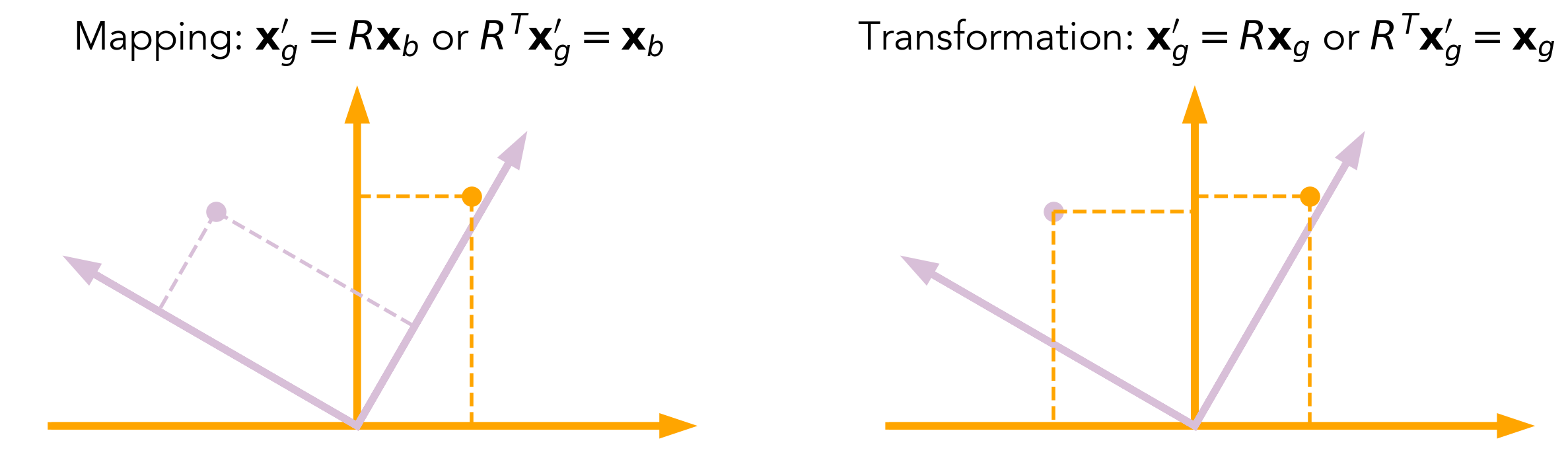
Rotation matrices can be seen as a mapping from describing a point in one coordinate frame to describing it in another coordinate frame. For the equation \(x_g^\prime = Rx_b\), we can see \(x_b\) as a point specified in a body frame \(b\) and \(x_g^\prime\) as the same point, specified in the coordinates of the global fixed frame \(g\). The rotation matrix \(R\) then serves as a mapping between these two representations.

Another way to see rotation matrices is to see them as an action that rotates points in the same frame from one configuration to another. Using the equation \(x_g^\prime = Rx_g\), we can see \(x_g\) as the point before applying the rotation \(R\) and \(x_g^\prime\) as the point after applying rotation \(R\).

With these two views, we can now better understand how to represent rotations w.r.t. the global fixed frame and the body frame. Now we ask: if we sequentially apply two rotations \(R_1\) and \(R_2\), both specified in the body frame, where would the point end up in the global frame? Denoting \(x_2\) as the final position in the global frame and \(x_0\) as the initial position in the global frame, we want to find the rotation matrix between \(x_2\) and \(x_0\). First, we denote the initial position in the global frame as \(x_0^g\), where the superscript \(g\) denotes that this is represented in the global frame. After applying \(R_1\), we have

\[x_1^g = R_1x_0^g.\]

One thing to note is that, in the body frame, the coordinates of the point are always the same, equal to \(x_0^g\). Thus, we have

\[R_1^Tx_1^g = x_1^{1} = x_0^g,\]

where the superscript \(1\) denotes the point represented in the body frame after rotation \(R_1\). If we see \(R_1\) as a mapping between points in frame \(1\) and the global frame \(g\), we have the following relationship

\[R_1^Tx^g = x^{1}\ \mathrm{and}\ x^g = R_1x^{1}.\]

Then we can see that if we apply \(R_2\), which is w.r.t. the frame \(b1\), we have

\[x_2^{1} = R_2x_1^{1}\ \rightarrow\ R_2^Tx_2^{1} = x_2^{2} = x_1^{1} = x_0^g;\]

similar to before, this utilizes the fact that the coordinates of the point are kept constant in the current body frame. Finally, if we use \(R_1\) to map \(x_2^{1}\) to \(x_2^g\), we have

\[R_1x_2^{1} = x_2^g;\]

then we can have

\[x_2^{g} = R_1R_2x_0^{g}.\]

An interesting question would be: after we get \(x_2^{g}\), if we rotate about the global frame using \(R_3\) and then rotate about the body frame using \(R_4\), what point will we end up at? If we call the point after applying \(R_3\) \(x_3\), we can easily have

\[x_3^g = R_3x_2^g = R_3R_1R_2x_0^{g} = R_3R_1R_2x_3^{3},\]

which again utilizes the fact that the body frame coordinates do not change: \(x_3^{3} = x_2^{2} = x_1^{1} = x_0^g\). We also obtain a mapping between the global frame and body frame \(3\): \(x^g = R_3R_1R_2x^3\). Then if we apply \(R_4\) and get to point \(4\), we have

\[x_4^{3} = R_4x_3^{3}\ \rightarrow\ R_4^Tx_4^{3} = x_3^{3} = x_4^{4} = x_0^g.\]

To map \(x_4^{3}\) into the global frame, we have

\[R_3R_1R_2x_4^{3} = R_3R_1R_2R_4x_4^{4} = x_4^g\ \rightarrow\ R_4^TR_2^TR_1^TR_3^Tx_4^g = x_0^g\ \rightarrow\ x_4^g = R_3R_1R_2R_4x_0^g.\]

Following this line of thought, I conjecture that we can completely decouple the rotations about the global frame and the body frame. I am pretty sure this is proved and shown somewhere; if anyone reading this has any information, please let me know.

Rigid Motions in 3D

In this section, I will talk about rigid motions, which include both translation and rotation. I will present three ways of describing such a motion, namely, homogeneous transformations, twists, and screw motions, and we will see how these three descriptions are related.

Homogeneous Representations

Any rigid motion can be represented by a translation \(p\) and a rotation \(R\). If we perform such a transformation \(g(\cdot)\), we can relate the position before and after the transformation as

\[q^\prime = g(q) = p + Rq.\]

And for a vector \(v\), we have \(g_*(v) = Rv\). This forms the special Euclidean group

\[SE(3) = \{(p, R)\ |\ p\in\mathbb{R}^3, R\in SO(3)\} = \mathbb{R}^3\times SO(3).\]

As before, we can see this in two ways. If \(g(\cdot)\) is seen as an action, then both \(q^\prime\) and \(q\) are measured in the same coordinate frame. If we see this as a mapping between frames, then \(q^\prime\) and \(q\) are measured in different frames. Later I will consolidate this using an example. Before that, I want to introduce the homogeneous representation of points and vectors. For a point \(p\) and a vector \(v\), we can have their homogeneous representations as \(\bar{p} = \begin{bmatrix} p_1\\ p_2\\ p_3\\ 1 \end{bmatrix},\ \bar{v} = \begin{bmatrix} v_1\\ v_2\\ v_3\\ 0 \end{bmatrix};\)

here I would like to draw your attention to the last element: for points, the last element is \(1\); and for vectors, the last element is \(0\). Then we can write the homogeneous representation of \(SE(3)\) as

\[\bar{g} = \begin{bmatrix} R & p\\ \mathbf{0} & 1 \end{bmatrix}.\]

It can be proved that \(SE(3)\) is a group; therefore, it satisfies the following properties:

If \(g_1, g_2\in SE(3)\), then \(g_1g_2\in SE(3)\).
It has an identity element, which is \(I_{4\times4}\).
There exists an inverse for \(g = (p, R)\in SE(3)\), defined as \(g^{-1} = (-R^Tp, R^T)\ \rightarrow\ \bar{g}^{-1} = \begin{bmatrix} R^T & -R^Tp\\ \mathbf{0} & 1 \end{bmatrix}.\)
The composition rule \(\bar{g}_{ac} = \bar{g}_{ab}\bar{g}_{bc} = \begin{bmatrix} R_{ab}R_{bc} & R_{ab}p_{bc} + p_{ab}\\ \mathbf{0} & 1 \end{bmatrix}\) is associative.

Also, we can prove that it is a rigid transformation, which implies

\(g\) preserves the distance between points: \(\|g(p) - g(q)\| = \|p - q\|\), for all \(p, q\in\mathbb{R}^3\).
\(g\) preserves the orientation between vectors: \(g_*(v\times w) = g_*(v)\times g_*(w)\), for all \(v, w\in\mathbb{R}^3\).

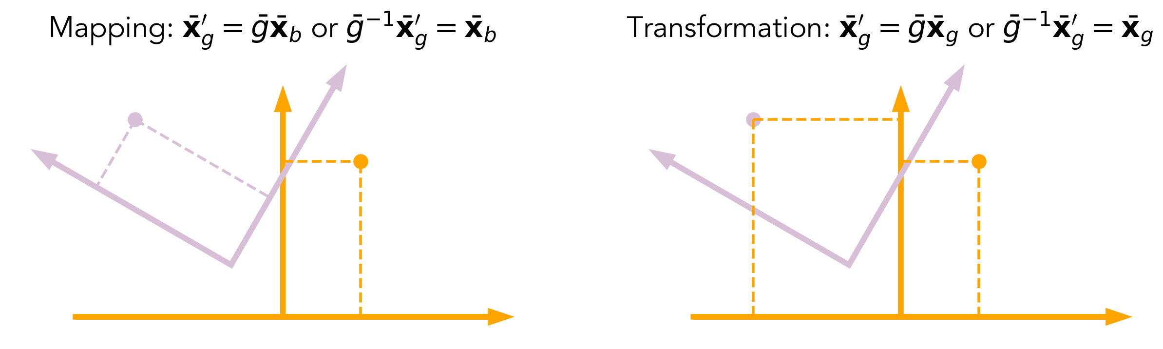
Now I want to use an example to better understand the two views of this homogeneous representation. Consider rotating by \(\theta\) about the vertical line going through point \((l_x, l_y, 0)\). How can we find the transformation \(g_{ab}\) such that \(x_g\) is the position of the point before and \(x_g^\prime\) is the position after, both represented in the global fixed frame? We can see this as two steps: a rotation \(R\) and a translation \(p\), where the rotation is w.r.t. the vertical line at \((0, 0, 0)\) and the translation is from \((0, 0, 0)\) to \((l_x, l_y, 0)\). Denoting a point \(x\) with its coordinates in the body frame (light purple frame above) as \(x_b\), we define

\[x_b^1 = Rx_b.\]

And after the translation, we have

\[x_g^\prime = x_b^1 + p = Rx_b + p.\]

Therefore, we have

\[x_g^\prime = p + Rx_b\ \rightarrow\ \bar{g} = \begin{bmatrix} R & p\\ 0 & 1 \end{bmatrix} = \begin{bmatrix} \cos\theta & -\sin\theta & 0 & l_x\\ \sin\theta & \cos\theta & 0 & l_y\\ 0 & 0 & 1 & 0\\ 0 & 0 & 0 & 1 \end{bmatrix}.\]

Also, if we start at point \(x_g = x_b\), where \(x_g\) is measured in the global frame, this gives us a way to calculate the position after applying \(R\) and \(p\):

\[x_g^\prime = p + Rx_g.\]

Twists

In the previous sections, we talked about how to rotate rigid bodies; however, all of them were rotating about an axis that passes through the global fixed frame. In this part, in addition to introducing a more compact way of representing rigid body motion, I will also talk about how to rotate about axes that do not pass through the origin of the fixed frame. In homogeneous coordinates, we can write a pure rotation with unit velocity about an axis \(\omega\in\mathbb{R}^3\)

\(\dot{p}(t) = \omega\times(p(t) - q)\) as \(\begin{bmatrix} \dot{p}\\ 1 \end{bmatrix} = \begin{bmatrix} \hat{\omega} & -\omega\times q\\ 0 & 1 \end{bmatrix}\begin{bmatrix} p\\ 1 \end{bmatrix} = \hat{\xi}\begin{bmatrix} p\\ 1 \end{bmatrix}\ \longleftrightarrow \dot{\bar{p}} = \hat{\xi}\bar{p}.\)

Thus, the solution \(\bar{p}(t) = \exp{(\hat{\xi}t)}\bar{p}(0)\) enables a mapping from the initial location to the location after \(t\) radians of rotation via \(\exp{(\hat{\xi}t)}\). Note that here \(q\) is a point on the axis \(\omega\) given in the global coordinates. For pure translations, we have

\[\hat{\xi} = \begin{bmatrix} 0 & v\\ 0 & 0 \end{bmatrix}\]

where \(v\) is a vector representing the translation velocity. We define twists as the group:

\[\hat{\xi} \in se(3) := \{(v, \hat{\omega})\ |\ v\in\mathbb{R}^3, \hat{\omega}\in so(3)\} = \begin{bmatrix} \hat{\omega} & v\\ 0 & 1 \end{bmatrix}\in\mathbb{R}^{4\times4},\]

with the twist coordinates \(\xi := (v,\ \omega)\). We can prove that for every member of \(se(3)\), we can find its corresponding element in \(SE(3)\) using an exponential mapping

\[\begin{align*} e^{\hat{\xi}\theta} &= \begin{bmatrix} I & v\theta\\ 0 & 1 \end{bmatrix} & \omega = 0\\ e^{\hat{\xi}\theta} &= \begin{bmatrix} e^{\hat{\omega}\theta} & (I - e^{\hat{\omega}\theta})(\omega\times v) + \omega\omega^Tv\theta\\ 0 & 1 \end{bmatrix} & \omega \neq 0. \end{align*}\]

Also, for every \(p, R\), we can find a corresponding twist \(\hat{\xi}\in se(3)\) and \(\theta\in\mathbb{R}\); for \(R = I\), we have

\[\begin{align*} \hat{\xi} &= \begin{bmatrix} 0 & p/\|p\|\\ 0 & 0 \end{bmatrix} &\theta = \|p\|. \end{align*}\]

If \(R \neq I\), then first we can solve for \(\hat{w}\) and \(\theta\) by solving \(e^{\hat{\omega}\theta} = R\), which was mentioned above. Then we can solve for \(v\):

\[v = \Big[(I - e^{\hat{\omega}\theta})\hat{\omega} + \omega\omega^T\theta\Big]^{-1}p.\]

Note that here, if we write \(p(\theta) = \exp{(\hat{\xi}\theta)}p(0)\), then \(p(\theta)\) and \(p(0)\) are specified in the same reference frame. If we want to specify \(p(0)\) in the body frame, then we have

\[p(\theta) = \exp{(\hat{\xi}\theta)}g_{gb}(0)p^b(0),\]

where \(g_{gb}\) gives the mapping between coordinates in the body frame and the global frame at \(t = 0\).

Twist	Linear System	Comments
\(\dot{p}(t) = \omega\times(p(t) - q)\)	\(\dot{x}(t) = \omega(x(t) - O)\)	\(\xi = \begin{bmatrix}-\omega\times q\\ \omega\end{bmatrix} = \begin{bmatrix}v\\ \omega\end{bmatrix}\), differential equations governing the movement
\(\dot{\bar{p}} = \hat{\xi}\bar{p}\)	\(\dot{x} = Ax\)	\(\hat{\xi} = \begin{bmatrix}\hat{\omega} & -\omega\times q\\ 0 & 1\end{bmatrix}\), differential equation in vector form
\(\bar{p}(t) = \exp{(\hat{\xi}t)}\bar{p}(0)\)	\(x(t) = \exp{(At)}x(0)\)	\(\exp{(\hat{\xi}t)} = \begin{bmatrix}e^{\hat{\omega}\theta} & (I - e^{\hat{\omega}\theta})(\omega\times v) + \omega\omega^Tv\theta\\ 0 & 1\end{bmatrix}\), analytic solution to differential equation.

Screw Motion

Here we state Chasles’ Theorem: every rigid body motion can be realized by a rotation about an axis \(\omega\) combined with a translation parallel to that axis. We assume that the rotation is by \(\theta\) radians and the translation is by an amount \(d\); we can also find a point on \(\omega\) and call it \(q\).

We can see that this movement resembles the movement of a screw. We can describe the screw movement using: the pitch as \(h:=d/\theta\), the axis of the screw movement as

\[l = \{q + \lambda\omega\ |\ \lambda\in\mathbb{R}\},\]

and a magnitude \(M = \theta\) when there is rotation and \(M = \infty\) when there is only translation.

For a given screw motion, we can find its rigid transformation as

\[\begin{align*} g &= \begin{bmatrix} e^{\hat{\omega}\theta} & (I - e^{\hat{\omega}\theta})q + h\theta\omega\\ 0 & 1 \end{bmatrix} & \mathrm{with\ rotation}\\ g &= \begin{bmatrix} I & \theta v\\ 0 & 1 \end{bmatrix} & \mathrm{pure\ translation} \end{align*}\]

where \(v\) is the vector of translation. Additionally, when given a twist, we can also find its corresponding screw, and given a screw, we can find its corresponding twist.

Velocity of a Rigid Body

Rotational Velocity

First, we define the spatial coordinate frame \(A\), which is fixed, and the body coordinate frame \(B\), which is moving. If we define a point \(q_b\) in the body frame and a rotational motion \(R_{ab}(t)\), then we can have the trajectory of the point in spatial coordinates as

\[q_a(t) = R_{ab}(t)q_b.\]

By deriving that both \(R^{-1}\dot{R}\) and \(\dot{R}R^{-1}\) are skew-symmetric matrices, we can get the angular velocity in both the spatial coordinates \(\hat{\omega}^s\) and the instantaneous body coordinates \(\hat{\omega}^b\) (since the body coordinate frame is changing due to rotation)

\[v_{q_a}(t) = \dot{R}_{ab}(t)q_b = \underbrace{\dot{R}_{ab}(t)R_{ab}^{-1}(t)}_{:=\ \hat{\omega}_{ab}^s}R_{ab}(t)q_b = \hat{\omega}_{ab}^sR_{ab}(t)q_b = \hat{\omega}_{ab}q_a.\]

The instantaneous body angular velocity is defined as seeing the spatial angular velocity vector in the body frame,

\[v_{q_b}(t) := R_{ab}^Tv_{q_a}(t)\ \ \ \ \hat{\omega}_{ab}^b = R_{ab}^{-1}\dot{R}_{ab},\]

which is not the angular velocity of the rigid body w.r.t. the body frame; the latter is always zero.

Rigid Body Velocity

For a rigid motion plan \(g_{ab}(t)\in SE(3)\), we can get the spatial velocity as a twist \(\hat{V}_{ab}^s\in se(3)\)

\[\hat{V}_{ab}^s = \dot{g}_{ab}g_{ab}^{-1}\ \ \ \ V_{ab}^s = \begin{bmatrix} v_{ab}^s\\ \omega_{ab}^s \end{bmatrix} = \begin{bmatrix} -\dot{R}_{ab}R_{ab}^Tp_{ab} + \dot{p}_{ab}\\ (\dot{R}_{ab}R_{ab}^T)^\vee \end{bmatrix}\]

Thus, the velocity of a point \(q_a\) can be found as

\[v_{q_a} = \hat{V}_{ab}^sq_a = \omega_{ab}^s\times q_a + v_{ab}^s.\]

Here we can interpret \(\omega_{ab}^s\) as the instantaneous angular velocity of the body as viewed in the spatial frame, and \(v_{ab}^s\) as the velocity of a (possibly imaginary) point on the rigid body that is traveling through the origin of the spatial frame at time \(t\). The body velocity is defined as

\[\hat{V}_{ab}^b = g_{ab}^{-1}\dot{g}_{ab}\ \ \ \ V_{ab}^b = \begin{bmatrix} v_{ab}^b\\ \omega_{ab}^b \end{bmatrix} = \begin{bmatrix} R_{ab}^T\dot{p}_{ab}\\ (R_{ab}^T\dot{R}_{ab})^\vee \end{bmatrix}\]

where \(v_{ab}^b\) can be interpreted as the velocity of the origin of the body coordinate frame relative to the spatial frame, as viewed in the current body frame; and \(\omega_{ab}^b\) can be seen as the angular velocity of the coordinate frame, also as viewed in the current body frame. We can also define an adjoint transformation to relate the spatial and body velocities:

\[V_{ab}^s = \begin{bmatrix} v_{ab}^s\\ \omega_{ab}^s \end{bmatrix} = \begin{bmatrix} R_{ab} & \hat{p}_{ab}R_{ab}\\ 0 & R_{ab} \omega_{ab}^b \end{bmatrix}\begin{bmatrix} v_{ab}^b\\ \omega_{ab}^b \end{bmatrix} = Ad_{g}V_{ab}^b.\]

Coordinate Transformation

For three coordinate frames \(A\), \(B\), and \(C\), we can have the relationship between their spatial velocities as

\[V_{ac}^s = V_{ab}^s + Ad_{g_{ab}}V_{bc}^s;\]

similarly, we can get the relationship between their body velocities as

\[V_{ac}^b = Ad_{g_{bc}^{-1}}V_{ab}^b + V_{bc}^b.\]

This relationship can also be used to represent twists before and after applying a rigid motion:

\[\xi^\prime = Ad_g\xi\ \ \mathrm{or}\ \ \hat{\xi}^\prime = g\hat{\xi}g^{-1}.\]

Some additional properties include:

\[\begin{align*} V_{ab}^{b} &= V_{ba}^{s}\\ V_{ab}^{b} &= -Ad_{g_{ba}}V_{ba}^{b} \end{align*}\]

Wrenches

A wrench is defined as a force/moment pair \(F\in\mathbb{R}^6\):

\[F = \begin{bmatrix} f\\ \tau \end{bmatrix}.\]

Given its dual nature with a twist, we have the relationship mapping wrenches between different coordinate systems as

\[F_c = Ad_{g_{bc}}^TF_b.\]

For the same wrench, the instantaneous work is the same in both the spatial and body frames:

\[\delta W = V^b\cdot F^b = V^s\cdot F^s,\]

where \(\cdot\) represents the dot product.

Using Poinsot’s Theorem, we can see that every collection of wrenches applied to a rigid body is equivalent to a force applied along a fixed axis plus a torque about the same axis. Thus, there exists a direct mapping between wrenches and screw motions.